Choosing an appropriate file format is essential, whether your data transits on the wire or is stored at rest. Each file format comes with its own advantages and disadvantages. We covered them in a precedent article presenting and comparing the most popular file formats in Big data. In a follow up article, we will compare their performance according to multiple scenarios. The compression used for a given format greatly impact the query performances. This article will prepare the tables needed for this follow up article and takes the opportunity to compare the compression algorithms in terms of storage spaces and generation time. It will also helps us to select the most appropriate compression algorithms for each format.
Database Choice
Apache Hive is a Data Warehouse software built on top of Hadoop. It is used to manage large datasets using SQL syntax. We choose it for the following reasons:
- Hive is designed for analytical tasks (OLAP).
- It can take fully advantage of the distributed data processing. It supports several types of file formats.
- In some circumstances, using an optimized language like HiveQL present the advantage of preventing the code execution from human mistakes and enables potential engine optimizations.
- HiveQL being based on SQL, is an declarative language which makes the model definition and the query declaration easy to express and to read.
Note, it would have been possible to use an alternative execution engine such as Apache Spark.
Characteristics of the cluster and datasets
Our environment is running the HDP distribution 3.1 from Hortonwork and now distributed by Cloudera. In order to better assess the raw performance of file format, it is relevant to work on a relatively large data set. At least 10 GB is to be considered the minimum, a few hundred of GBs would be much more relevant.
We selected 3 datasets with different characteristics to evaluate the behaviors of the selected file formats on different data structures:
- NYC taxi is a time series data. The datasets contain trip and fare data represented from 2010 to 2013. The raw data of trip have about 86.8 GB and fare takes up 49.9 GB.
- IMDB is a relational data. It provides seven tables in TSV format:
imdb.name.basics,imdb.title.basics,imdb.title.crew,imdb.title.akas,imdb.title.ratings,imdb.title.episodeandimdb.title.principals. Their total size in uncompressed format is 4.7 GB. Nevertheless we will not assess this dataset du to its small size(less than 10GB), notice that it will be helpfull for our next article when assessing the performance of these datasets with their various codecs in HiveQL. - Wikimedia is a semi-structured data with a complex structure (nested data). It takes up 43.8 GB of uncompressed data in JSON format.
Load data in HDFS
The following script shows how to download datasets directely into hdfs.
source='http://...'
hdfs dfs -put <(curl -sS -L $source) /user/$env:USER/dataset
Schema declaration in Hive
The NYC Taxi dataset is made of two tables:
SET hivevar:database=<DATABASE NAME>;
USE $database;
DROP TABLE IF EXISTS trip_data;
CREATE EXTERNAL TABLE trip_data
(
medallion NUMERIC, hack_license NUMERIC, vendor_id STRING, rate_code NUMERIC,
  store_and_fwd_flag NUMERIC, pickup_datetime STRING, dropoff_datetime STRING,
  passenger_count NUMERIC, trip_time_in_secs NUMERIC, trip_distance NUMERIC,
  pickup_longitude NUMERIC, pickup_latitude NUMERIC, dropoff_longitude NUMERIC,
  dropoff_latitude NUMERIC
)
ROW FORMAT DELIMITED
FIELDS TERMINATED BY ","
STORED AS TEXTFILE
LOCATION "/user/$username/trip_data/"
TBLPROPERTIES ("skip.header.line.count"="1");
DROP TABLE IF EXISTS trip_data;
CREATE EXTERNAL TABLE fare_data
(
  medallion NUMERIC, hack_license NUMERIC, vendor_id STRING, pickup_datetime STRING,
  payment_type STRING, fare_amount NUMERIC, surcharge NUMERIC, mta_tax NUMERIC,
  tip_amount NUMERIC, tolls_amount NUMERIC, total_amount NUMERIC
)
ROW FORMAT DELIMITED
FIELDS TERMINATED BY ','
STORED AS TEXTFILE
LOCATION '/user/$username/fare_data/'
TBLPROPERTIES ("skip.header.line.count"="1");
The Wikimedia dataset is made of one table:
SET hivevar:database=<DATABASE NAME>;
USE $database;
DROP TABLE IF EXISTS wiki_data_json;
CREATE EXTERNAL TABLE wiki_data_json
(
  id STRING, `type` STRING,
  aliases MAP<string, array<struct<language:string, value:string>>>,
  descriptions MAP<string, struct<language:string, value:string>>,
  labels MAP<string, struct<language:string, value:string>>,
  claims MAP<string, array<struct<id:string, mainsnak:struct<snaktype:string, property:string,
  datatype:string, datavalue:struct<value:string, type:string>>, type:string, `rank`:string>>>,
  sitelinks MAP<string, struct<site:string, title:string, badges:string>>
)
ROW FORMAT SERDE "org.openx.data.jsonserde.JsonSerDe"
WITH SERDEPROPERTIES ("ignore.malformed.json"="true", "skip.header.line.count"="1")
STORED AS TEXTFILE
LOCATION "/user/$username/Wikimedia/";
Our tables are declared in Hive as external. This allows us to define a table which is not managed by Hive. Here are two simple queries to ensure our table are declared and our data are readable:
use $database;
show tables;
SELECT * FROM trip_data LIMIT 10;
Converting data into another file format
Each conversion is tested with and without compression. This is done in ORC, Parquet, CSV, JSON and AVRO formats. In Hive, the CSV format can be declared in different manner, either using CSV Serde or CSV simplified format from TEXTFILE formats. The first includes all the characteristics related to CSV format such that the separator, quote and escape characters. However, it contains a limitation by treating every columns as a string type. The second was used instead. While the CSV implementation is more naive, it preserves the native data type of each columns.
File formats can support all or a selected list of compression algorithms called codecs. For example, ORC and Parquet respectively default to ZLIB and GZIP and both additionnaly support Snappy. Text file formats have no restriction on the compression being applied. The available codecs are limited by what the data warehouse supports. In our case, there are different types of compression supported in Hive. In addition to Snappy and gzip, we choose to test bzip2 and lz4. For AVRO, we choose to also test the Deflate codec in addition to Snappy but more codecs are supported.
In order to automate this process, we wrote a bash script which creates and retrieves the metrics before deleting the table.
username=`whoami`
for i in /home/$username/requests_file/*;
do
metrics_file="$(echo "$i" | awk -F"/" 'print $NF')"."csv"
sh <<EOF
beeline -u "jdbc:hive2://zoo-1.au.adaltas.cloud:2181,zoo-2.au.adaltas.cloud:2181,zoo-3.au.adaltas.cloud:2181/dsti;serviceDiscoveryMode=zooKeeper;zooKeeper$"
 -f "$i" 2>&1 | awk '/^[INFO].*VERTICES.*$/||/^[INFO].*Map .*$/||/^[INFO].*Reducer .*$/' >> "$metrics_file"
EOF
hdfs dfs -du -s -h /user/$username/tables/* >>"$metrics_file"
hdfs dfs -rm -r -skipTrash /user/$username/tables/*
done
An example of the $i variable could be:
CREATE EXTERNAL TABLE trip_data_orc
(
)
STORED AS ORC
LOCATION '/user/$env:USER/trip_data/trip_data_orc'
TBLPROPERTIES ("orc.compress"="ZLIB");
SET hive.exec.compress.output=true;
insert into trip_data_orc
select * from trip_data;NOTE:
- Make sure that the folder
/home/$username/requests_file/contains the queries as the above example. - The command to retrieve the storage space generates two columns. The first column provides the raw size of the files in HDFS directories. The second column indicates the actual space consumed by these files in HDFS. The second column provides a value much higher than the first due to replication factor configured in HDFS.
- We deliberately choose to not convert the Wikimedia dataset into CSV because of its structure which does not perfectly fit the CSV constrains.
- For more reliability, these tests were done on three repetitions. The final result described in the next section is represented by the mean value.
Results
Our script generated some metrics we have formatted in the following tables:
Interpretation
We will analyze the results in various angles. The storage ratios are relative to the uncompressed JSON file format used as a reference.
Outliers of Parquet
We note that Parquet compression algorithm is not working. This may be due to the absence of some snappy compression jar files in the HDP platform.
Analysis by file format
We will analyze the formats independently and try to highlight advantages to use a format depending on specific use cases.
JSON
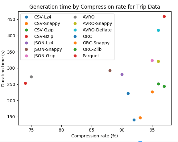
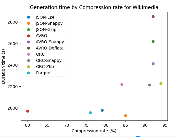
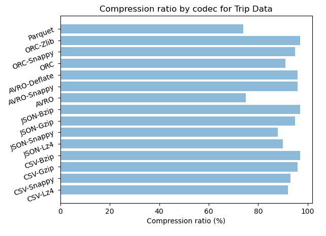
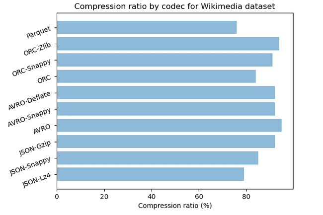
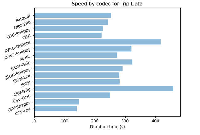
For JSON format we notice that the compression has a strong impact between 90% and 97% for trip data and between 79% and 95% for wikimedia. We can notice that compression algorithms with JSON are less performant with semi structured dataset. In terms of speed compression algorithms with JSON are fast but we can observe that higher is the compression rate slower is the algorithm.
AVRO
With AVRO we have strong compression rate with 92% for wikimedia and 96% for trip data. It also has an acceptable speed regarding his compression performance. Compression algorithms with AVRO are more efficient with time series dataset that have a lot of floats.
ORC
With ORC we have very strong compression rate up to 97% for trip data and 94% for wikimedia. The generation time is lower than for other format and it is less CPU consuming. For datasets with lot of float and sparse columns like trip data dataset, ORC’s compression algorithms are very efficient.
PARQUET
In its uncompressed form Parquet have a storage ratio of 74% for trip data and 76% for wikimedia compared to JSON. Parquet seems to be more efficient with dataset that have a lot of text.
Analysis of row based formats
For trip data which is time series dataset made of float values we can see that the different codecs give us almost the same compression rate between 92% and 97% for CSV, between 88% and 97% for JSON and 96% for AVRO. Bzip codec is slightly stronger than Gzip but the later is twice faster when applied with CSV and six times faster with JSON format. AVRO-Snappy and AVRO-Deflate have the same compression rate but the former is slightly faster.
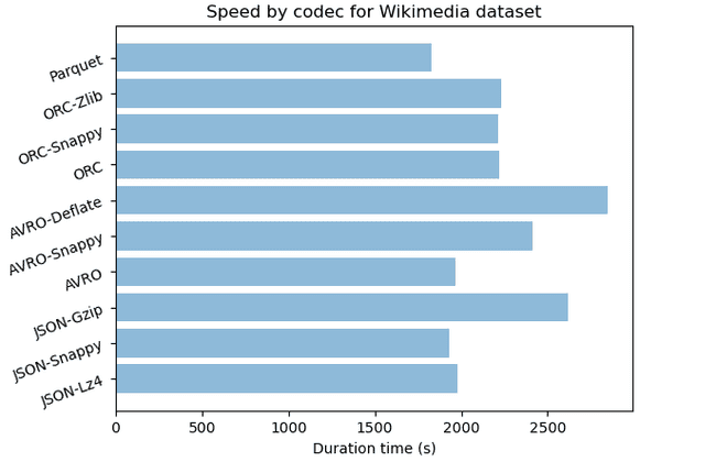
For Wikimedia which is a semi structured dataset with lot of text, JSON-Bzip is very efficient with 95% of compression rate. JSON-Gzip and JSON-Snappy are very close with respectively 92% and 85%. AVRO with Snappy and Deflate codecs has a strong compression of 92%. Eventhought JSON-Bzip is slightly stronger, JSON-Gzip and AVRO with Snappy are three times faster.
For semi structured data if you look for strong compression consider strong algorithm like Bzip with JSON or CSV. But moderatly strong algorithm like Gzip with JSON or Snappy with AVRO are faster and give almost the same storage ratio. Example: for archiving, gzip could be a relevant choice since it will process faster the compression and provides a storage space not too far from bzip2.
AVRO itself has as default codec format deflate and could be additionally compressed by bzip2, snappy, xz and zstandard. It supports in hive deflate and Snappy compression where both were tested. From our results, we have good compression rate in both datasets and we can note that snappy has a faster compression speed than deflate.
JSON vs AVRO
Let’s compare JSON and AVRO that are format widely used for data exchange between systems, programming languages, and processing frameworks. In their uncompressed form JSON that is a text based format is larger than AVRO that is a binary based format. AVRO occupies just quater JSON for trip data that is a time series dataset and just 40% of JSON for wikimedia that is a semi structured dataset.
AVRO is very compact and fast. For stream data It has the advantage of having a schema defined in JSON that clearly specifies the structure. With a schema, data can also be encoded more efficiently. Thus, it is relevant to use it for stream data. JSON does not provide a schema that leads to verbosity and make it difficult for producers and consumers to understand each other.
Analysis of column based format
With column based format we have a high compression rate for all codecs with up to 97% of compression for ORC. ORC-zlib gives in both datasets an efficient compression rate of 97% and 94% and with ORC-Snappy 95% and 91%. The generation time for both codecs is almost the same with a slight advantage for ORC with Snappy.
We can notice that the compression is more efficient with time series dataset. ORC-Zlib is stronger but ORC-Snappy is faster in both semi structured and time series datasets.
Analysis by compression algorithms
In this section we will compare file format when the same algorithm is applied.
Bzip gives the same compression performance 97% with CSV and JSON, but the algorithm is four times faster with CSV format. Example for archiving we can consider store the dataset in CSV and apply Bzip codec as it will process faster and give the same storage performance.
Lz4 with CSV and JSON gives respectively 92% and 90% of compression rate. Lz4 with CSV is twice faster than JSON.
- CSV-Snappy vs JSON-Snappy vs AVRO-Snappy vs ORC-Snappy vs Parquet-Snappy
Compression rate are very close for all format but we have the higher one with AVRO around 96%. In terms of speed it is faster with CSV and ORC. The former is twice faster compared to JSON and AVRO. If we are looking for strong compression choose AVRO with Snappy and for speed consideration ORC with snappy is preferable.
Gzip has a high compression ratio around 95% with CSV and JSON. Their speed are close with a slight advantage for CSV.
Selection criteria of file format and codec
Now, how to choose an algorithm of compression for our datasets? Depending on our objective and constraints we can have various options.
Row vs Column format: with compression
For row based format bzip codec offers the higher compression rate of 97% for CSV and JSON, gzip follows closely with respectively with 96% and 92% for CSV and JSON.
For column based format ORC with zlib give in both datasets an efficient compression rate of 97% and 94% and with snappy 95% and 91%.
Both text based and column based have strong algorithms that produce almost similar results in term of storage.
When you need a strong compression
ORC-Zlib, JSON-Bzip and CSV-Bzip give the same compression rate of 97%. ORC-Zlib is twice faster than CSV-Bzip and eight times faster than JSON-Bzip. For archiving ORC with Zlib is the best choice for column based format and CSV with Bzip is preferable for text based format.
When you need a fast processing
Lz4, Snappy, Gzip, Zlib are the fastest algorithms. It can be seen that the faster the algorithm, the less efficient it is in compression. These algorithms are more efficient when applied to row based formats. For column based format ORC with Snappy is the fastest algorithm and for text based format you can consider Lz4 or Snappy.
Conclusion
Through this study, we got an insight of how each file formats behaves in terms of compression and generation speed. Other aspect such as how they performs queries will be considered in our next article.
We can conclude by saying that columnar formats optimize better storage resource than row or text based file formats. For archiving it is preferable to choose column based format and ORC. If you have to deal with text based format Bzip and Gzip codecs optimize better the storage and for column based format it is Zlib with ORC. ORC offers an efficient compression plus a columnar storage which leads to smaller disk reads. In terms of speed we have different behavior depending on the format. For instance, for text based format the speed seems to be correlated to the storage space. The higher is the gain of storage, the longer it takes to perform the compression task. But for Column based format the generation time remains low for strong compression algorithms.
